Dimensional Fact Modelling
You can use the following table of content to navigate around this topic:
General Information
Published in 1998, the Dimensional Fact Model by Golfarelli, Maio and Rizzi represents a graphical conceptual model for data warehouses. It was developed to fill the conceptual gap between the end-user's requirements and the logical or physical design of the data warehouse (see [GMR98a] and [GMR98b]).
Most existing enterprise OLTP (On-Line Transactional Processing) systems are based on relational databases, and in most cases were planned and documented using Entity/Relationship (E/R) schemas. However, the E/R model does not meet the requirements of multidimensional modeling as needed for the conceptual design of data warehouses. There have been various efforts to extend the E/R model to make it fit but without satisfying results.
The Dimensional Fact Model introduces a graphical notation focused on the concerns of data warehouse and OLAP (On-Line Analytical Processing).
"The DF model is a collection of tree-structured fact schemas whose basic elements are facts, attributes, dimensions and hierarchies; other features which may be represented on fact schemas are the additivity of fact attributes along dimensions, the optionality of dimension attributes and the existence of non-dimension attributes. Compatible fact schemas may be overlapped in order to relate and compare data." [GMR98a]
In addition to describing the capabilities of the Dimensional Fact Model the authors also propose a methodology to derive their model from existing E/R schemas.
Description of the Model
The Dimensional Fact Model represents the data warehouse as a set of tree-structured fact schemas describing the data-cubes.
Their core element is the fact, a focus of managerial interest like "sales of a sales agent". A fact is usually accompanied by certain key figures that measure the fact like "quantity sold", "returns" or "inventory level". They are referred to as fact attributes (aka key figures). However, a fact may also have no fact attributes at all. The fact and its attributes are represented by a box in the graphical model. (see Figure D.1)
The dimensions, displayed as circles directly attached to the fact, determine the finest level of information. Each combination of values of the dimensions is defined as a fact instance. In Figure D.1 there are three dimensions ("item", "sales agent", "month"), so each fact instance describes the quantity of a certain item sold during a certain month by a certain sales agent. The same applies to "returns". In the case of a fact without any fact attributes, each fact instance would only record the occurrence of the fact.
Hierarchies that are rooted in the dimensions determine the possible aggregation levels. The connection between two attributes within a hierarchy or between an attribute and the according dimension can be interpreted as a many-to-one relationship, e.g. each "item" belongs to exactly one "group". The relation between two attributes of a hierarchy may be optional, in this case it is tagged by a dash (it is helpful to indicate the optionality with regard to logical design). Attributes inside hierarchies are represented by circles.
There may also be non-dimension attributes. They carry additional information about an attribute and can not be used for aggregation, e.g. "weight" in Figure D.1. Non-dimension attributes are shown as lines instead of circles.
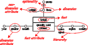
Figure D.1 - The fact schema
Please note that the highest level of aggregation (i.e. the summarization over all instances along one dimension, e.g. all "items") is not shown in the fact schema.
Types of Aggregation
By default, fact attributes are additive along all dimensions, e.g. if we move from the finest aggregation level "item" to the broader one "group", the fact attribute "quantity sold" is simply summed up for all "items" belonging to a certain "group". The same is valid for the other dimensions. We say fact attribute "quantity sold" is additive.
However, there is also the possibility of non- or semi-additive fact attributes. A typical example for a non-additive fact attribute would be a "temperature level". It doesn't make sense to add up two or more temperatures, one could choose "average" for aggregation instead of "summation" here. We speak of a semi-additive fact attribute if it is not additive along at least one dimension. In Figure D.2 "inventory level" is non-additive along dimension "month", but it is so along the others. Thus "inventory level" is semi-additive.
In the model semi-additivity is represented by a dotted line that connects the corresponding fact attribute to the dimensions along which it is non-additive. If another operator instead of sum can be used, it is explicitly indicated. Figure D.2 shows an example:
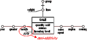
Figure D.2 - Semi-additivity
All of the above examples represent metric key figures, either with a rational or interval scale. However there are two other types that have not been mentioned yet: Nominal and ordinal key figures. An example for a nominal key figure would be a person's sex, ratings such as school marks represent ordinal ones.
The following table compares the different types of key figures and some of the operators that can be used on them:

Table D.1 - Types of key figures
Combining Fact Schemas
As quoted in the introduction, fact schemas may be overlapped if they are compatible, i.e. they have to share at least one dimension attribute.
Lets consider the following two fact schemas. The first one is our previous "sales agent" example. The other one contains data about courses our sales agents attend to improve their skills.
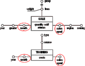
Figure D.3 - Overlapping two compatible fact schemas
These fact schemas are compatible, because they share the dimension attributes "sales agent" and "month". The resulting schema enables us to analyse the impact of training on sales.

Figure D.4 - The result from overlapping
Query Patterns
The dimensional fact model offers a notation to represent specific query patterns required by the end user. The query is represented by tagging the according dimension attributes. Within each hierarchy there may be no, one or more tags. Setting no tag at all means that the highest aggregation level is used, i.e. the fact attributes are summed up along this dimension. The result of a query may be any combination of fact attributes or the result of a computation on them. Figure D.5 shows the pattern for the following query: "Total quantity sold and average returns per unit sold for each item and for each quarter".
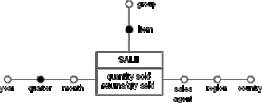
Figure D.5 - A query pattern
Deriving Fact Schemas from E/R-models
The data source for a data warehouse is usually an OLTP system based on a relational database. The widely used documentation method for relational data are E/R schemas, so it seems reasonable to derive the conceptual model of the warehouse from those.
The Dimensional Fact Model proposes a methodology consisting of five steps, that may not only be applied to E/R-schemas but also to other logical schemas, provided the cardinalities of the relations are known.
As a prerequisite we have to identify the facts of interest for the data warehouse, after that the following five steps have to be performed for each identified fact:
Building the attribute tree
Pruning and grafting the tree
Defining the dimensions
Defining the fact attributes
Defining hierarchies
The following E/R diagram will be used to build our sales fact schema:
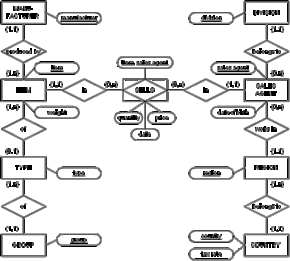
Figure D.6 - The underlying E/R schema for the sales agent example
Identifying Facts
As stated before, a fact is a focus of managerial interest, usually an event occurring dynamically.
In the E/R schema, facts are represented by entities or by relationships with a cardinality of n:m, the latter should be transferred into entities before carrying on. In our example, entity SELLS was originally a n:m relationship between ITEM and SALES AGENT (see [Hohe99] for a deeper consideration).
Now we can start selecting entities (or n:m-relationships converted to entities) as facts. Every identified fact becomes the root of a different fact schema.
Possible candidates for facts are frequently updated entities (like SELLS), more static entities like COUNTRY or MANUFACTURER may be ruled out. In our example the SELLS entity is chosen as the only fact.
1) Building the Attribute Tree
After identifying entity F as a fact the tree is built in the following way:
Each attribute and identifier (the primary key or the entity's name) within the E/R schema becomes a node (a node may represent a fact, a fact attribute (key figure), a dimension, a dimension attribute or a non-dimension attribute of the resulting fact schema)
The primary key of entity F becomes the root (grey)
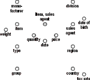
Figure D.7 - Primary keys and attributes
If a node corresponds to a primary key of an entity in the E/R schema, all other nodes representing attributes of this entity are attached to it.
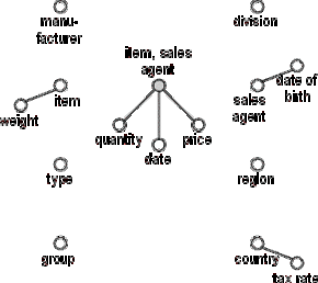
Figure D.8 - Connecting primary keys and corresponding attributes
The nodes representing primary keys are connected to each other according to their corresponding entity's relationships in the E/R schema. Optional relationships (i.e. relationships with a cardinality of (0,1) on the "1-side") are tagged by a dash.
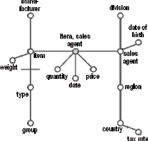
Figure D.9 - Connecting primary attributes according to relationships
After rearranging the nodes our attribute tree looks like this:
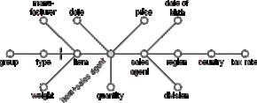
Figure D.10 - The result of step 1
2) Pruning and Grafting the Attribute Tree
Not all of the tree's attributes (nodes) may be of interest for the data warehouse, so the next step is eliminating unwanted or unnecessary information by pruning and grafting the attribute tree.
Pruning means to drop nodes or entire sub-trees. All attributes belonging to dropped sub-trees will not be included in the resulting fact schema and can therefore not be used as aggregation levels. In our example we could prune the entire sub-tree including "region", "country" and "tax rate" leaving us with only "division" as a possible higher aggregation level for "sales agent" ("date of birth" represents a typical candidate for a non-dimension attribute).
However, we decide to prune only "division", "date of birth" and "tax rate".
Grafting is used if a node or sub-tree contains unnecessary information but its descendants have to be preserved. We decide we only need a classification of the "items" by "group" and therefore graft "type". All descendants of a grafted attribute inherit its optionality.
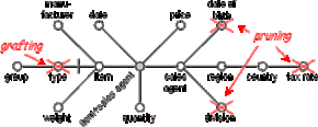
Figure D.11 - Pruning and grafting
It should be noted that grafting a child of the root decreases the granularity of data but increases the number of dimensions in the resulting fact schema if the grafted node has more than one descendant.
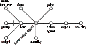
Figure D.12 - The attribute tree after pruning and grafting
3) Defining Dimensions
Defining dimensions is a key step, as they determine how the fact instances may be aggregated. They must be selected form the descendants of the root and may either be discrete attributes or ranges of discrete or continuous attributes.
In our example the attributes "item" and "sales agent" are good candidates for dimensions. Both are discrete attributes and the usage of a range is not necessary.
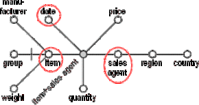
Figure D.13 - Defining dimensions
Time is usually a key dimension in the data warehouse, so we choose "months" (ranges of the "date" attribute) as a third dimension.
If the time-attribute appeared as a descendant of a node that is not the root, it would be necessary to consider grafting the attribute tree even more to make time become a dimension.
It is worth mentioning that there may be E/R schemas without any time-attributes at all. Those are snapshot schemas which just describe a current state. In this case old data is replaced continuously by new data in the OLTP. In the data warehouse however some kind of time-attribute may be added to store historical data and allow analysis over time.
After choosing the dimensions we are able to partially outline our fact schema.

Figure D.14 - First draft of the fact schema
4) Defining Fact Attributes
Fact attributes are usually the sum (or average, minimum or maximum) of expressions involving numerical attributes of the attribute tree that have not been chosen as dimensions. They may also be counts of the number of fact instances.
The existence of fact attributes is not compulsory. As stated in the description of the model a fact schema without any key figures may be meaningful, providing the occurrences of the fact are counted. If fact attributes are defined, it is helpful to create a glossary that describes how to calculate each key figure from the attributes of the E/R schema.
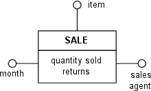
Figure D.15 - Draft of the fact schema with glossary
The sum operator in the glossary means that all fact instances are summed up for the same month, item and sales agent. If the E/R schema had "month" as its time attribute instead of "date", it would have been possible to translate the entity's attributes directly into the key figures of the fact schema without using any operators.
5) Defining Hierarchies
In the last step we define the hierarchies for the dimensions identified in step 3. Using the attribute tree we already have a meaningful basis for the organization of the hierarchies. It is still possible to further prune and graft the tree or to add additional aggregation levels, which is usually done for the time dimension. In our example we add "quarters" and "years" as ranges of "months".
Attributes that should not be used for aggregation but nevertheless provide important information may be tagged as non-dimensional. In our example this is the case for attribute "weight".
As we can see now the "item"-dimension in our example features a parallel hierarchy. The single "items" may be aggregated according to their "manufacturer" or the "group" they belong to.
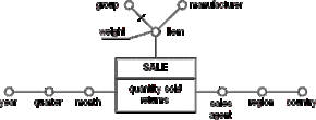
Figure D.16 - The resulting fact schema
Summary
The Dimensional Fact Model provides a database independent, conceptual view well suited for the dialog between the end-user and the data warehouse designer, the possibility to derive the model from existing E/R-schemas can greatly simplify the modeling task.
However a major disadvantage of the DFM and similar graphical representations is the way they depict data aggregation. Furthermore the Dimensional Fact Model becomes difficult to handle with a growing number of dimensions.
